Introduction:
When the MANIAC I computer defeated a human in a chess-like game for the first time in 1956, it was a monumental moment in history. The idea of machines being able to complete tasks by replicating how the human brain works started to gain hope and traction. Those, however, were tough times in which to even achieve discrete performance in other tasks due to the lack of data and computing power available.
Since then, a series of so-called “AI Winters” took place one right after another and the dream of computers performing at similar levels to humans had all but vanished entirely. It wasn’t until the beginning of 2005 that AI started to regain attention with Deep Learning as the singular force propelling its growth.
Today, companies are pouring billions of dollars into AI development and intelligent machines continue to participate in real world activities every day.
In this series of posts, we will review basic concepts about image manipulation, convolutional neural networks, and Deep Learning. We will then dive deeper into the computer vision field and train a Convolutional Neural Network to recognize cats and dogs in arbitrary images, all of this using the Python programming language, TensorFlow, and several other convenience packages. If you are new to TensorFlow, you can browse through its site and examples at https://www.tensorflow.org.
[Getting ready] Setting up our environment
Through this tutorial we will make use of the Python programming language, along with several other packages and tools, including Anaconda (conda) as our environment manager. We will follow these instructions to get our environment ready:
-
- Download and install Anaconda. It is available for free download at https://www.anaconda.com/download/.
- Once you’ve installed Anaconda, you will need to create a conda environment and add some packages to it. Let’s call it “deeplearning.” The following commands will complete the task:
|
Your environment should now be ready. Let’s test it by running the Jupyter Notebook and executing a simple “hello world” command:
|
Figure 1: Notebook with “hello world” message

[Warm up] Image processing: Filters and Convolutions
As we will be training and using a “convolutional” neural network, it is a good idea to understand why those types of networks are named what they are. Before we build our CNN model, we will recap some of the concepts needed in image processing.
A convolution is basically a mathematical operation of two functions, having the third one as the result. Convolutions are applied in several fields including image processing and computer vision.
In the field of image processing, a convolution matrix is used for image manipulation like blurring, sharpening, or edge detection. The original image is treated as a matrix with values from 0 to 255, according to the color intensity in each pixel. For grayscale images, this matrix will have only two dimensions: WxH (Width x Height). However, for color images using the RGB scheme there will be a third dimension. The matrix will become a structure with shape WxHx3 (Width x Height x 3 RGB Channels).
Image manipulation and convolutions in practice
Despite the formal definition and all the complicated maths behind convolutions for image processing, we can understand it as a relatively simple operation similar but not equal to matrix multiplication. Let’s see two classic examples with a grayscale image:
Image Equalization:
Before we start with convolutions, we’ll warm up by doing some basic image manipulation by equalizing a grayscale image.
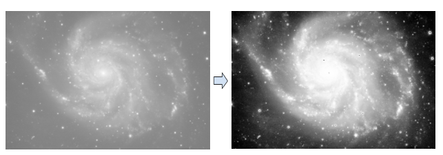
The image on the left has been acquired with a sensor (camera or telescope) and suffers from over-exposure. Therefore, it looks like there is too much lightness in the whole image. We need to enhance the image to the point where it looks like the one on the right side below:
Figure 2: Galaxy image before and after equalization

Performing exploration of the data we have is a recommended practice in almost any discipline. As we are given an image, calculating and visualizing its histogram seems to be the most common task to start with. To obtain our grayscale image histogram, we need to count how many pixels have an intensity of 0, 1, 2 and so on, up to 255, where 0 is a totally black pixel and 255 is a completely white one. Let’s code it:
# read the image in grayscale mode “L” |
After running the script above, we can see the histogram with a notable deviation to the right. The total of the pixels have values higher than 100. It is our goal to make the histogram look more evenly distributed or, more properly, equalize it.
Figure 3: Image histograms before and after equalization

The snippet below shows a simple algorithm that can be used to achieve the histogram equalization:
histogram_eq = histogram / (rows * cols) |
Now, to visualize the new equalized image, we need to convert the image_new array back to a grayscale image. Try it yourself!
Want a challenge? You can try applying a similar algorithm to equalize the following color image. While the principle is similar, one cannot just compute and equalize the three RGB channels independently.
Figure 4: Overexposed colorful image

Test the process yourself and show us what approach you used to address this challenge. We’d love to see your code and discuss your solution!
Image convolutions:
In our previous exercise we did a linear transformation on an image by simply modifying how the gray tones were distributed. However, that’s not all we can do with an image. Another modification we can make is replacing each pixel with the mean value of its neighbors, which is called a median filter. A median filter is a non-linear filter often used to reduce noise in images. You can read more about the median filter in this article in Wikipedia.
As we previously stated, a convolution is an operation between two functions to obtain a third one. In the image processing domain, the first function will be our original image and the second one will be a convolution matrix (also called Kernel or Filter matrix) with shape NxN where N is an even number frequently having values of 3, 5 or 7.
The animation below shows how we compute an output matrix as a result of performing a convolution with an input image matrix and a 3×3 kernel:
Animation 1: Convolution with a 3×3 Kernel

To obtain the modified image in the shape of a numerical matrix containing grayscale values, we start by taking a subsection of the input image with the same shape as our Kernel. Then, we perform element-wise multiplications between our input sample and kernel. Finally, we add the nine products and divide the result by the sum of all values in the kernel. The initial 320 value for our output matrix is, therefore, the result of the following operation:

Why do we have a top row and first column with zero values? The answer is that, in order to be able to perform the element-wise operation described before for the input elements at the border of our input matrix, we need to pad the original image with as many rows and columns as the size of our kernel matrix minus one, divided by two. So, in our example, our image will be padded with one column and one row because our kernel matrix size is three: (3-1)/2.
An important element is also introduced here and must be remembered for later: the strides. As we perform the operation in each pixel, we need to follow the same approach to visiting all the pixels in the original image, such as a sliding window. The stride will determine how many pixels we move to the right and to the bottom in each step. Most of the time the strides are one for both horizontal and vertical displacements.
You may also be wondering how one determines the shape the convolution kernel will have? There are several well-known kernels you can use for different purposes. Below you can see some of them and the result they produce when applied:

Now, let’s code it. Try it for yourself with this simple function for padding an image and performing a convolution with any kernel matrix:
def filter_simple(source, kernel, mask_rows, mask_cols): |
The function is as simple as:
# define our kernel |
Figure 5: Simple edge detection with convolution filters

There are a couple of places where you can improve the code. Have you also noticed that the execution isn’t as fast? Do you think you can improve it? Motivate yourself and read about optimization for convolution operations. Again, we’d love to see your code and discuss any question you may have.
Most image processing and numeric libraries that are in languages such as Python also offer ready-to-use optimized functions for 2D and 3D convolutions. Check out this example in the SciPy documentation!
[Finally] Discussion
Convolutions are a key concept to understand before we move to Convolutional Neural Networks as the kernel, strides, and other parameters have a lot of importance when dealing with them. In the next post, we will see how a neural network can learn its own kernels instead of using predefined ones. The ability to perform transformations such as noise reduction and edge detection that filters add is probably one of the biggest reasons CNN has become so popular and accurate.
References:
-
- Bengio, Y. (2016). Machines Who Learn. Scientific American, 314(6), 46-51. doi:10.1038/scientificamerican0616-46